[Page 6]
Utility of the respiratory tracing.
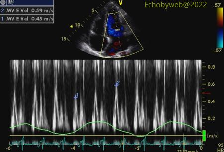
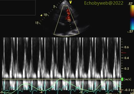
Examples of the use of respiratory tracing to monitor changes in flow velocities with respiration (pericardial diseases: constriction). Figure 20: before pericardiectomy (early expiratory increase: 31%). Figure 21: after pericardiectomy (no changes in flow with respiration).
See: Lesson on Pericardial physiology and pathology (Page 13.
Control of respiration.
- Increase the repeatability of the examination by acquiring the different views in the same condition. Respiration influences the hemodynamics of the heart, thus the standard is acquiring imaging at relaxed end expiration.
- In some situations, inspiration may increase visibility of certain cardiac structures (ex: the anterior wall of the left ventricle in the apical 2-chamber viewp), by displacing the heart upwards and towards the sternum.
Figure 22. No intervention. Figure 23. Imaging obtained at end-inspiration with additional repositioning of the transducer up one intercostal space (the transducer is now located on the anterior apex).
Origin of echocardiographic variability.
- Extrinsic factors (controllable)
– Moment of the day
– Medical therapy
– Postprandial status
– Phase of respiratory cycle - Biological factors (not easily controlable)
– “Adrenergic” state
– Arterial blood pressure
– Heart rate
- Technical factors
– Image acquisitioon
– Use of anatomical landmarks
– Adjustment of ultrasound gain
– Rigorous methodology
– Intra- and inter-operator variability
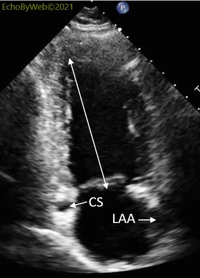
Use of anatomical landmarks. Apical LV 2-chamber view example: optimal imaging of the LV (Figure 24) is obtained by aligning 3 structures: 1. longest end-diastolic LV long axis; 2. cross-sectional view of the coronary sinus (CS); 3. visualization of the left atrial appendage (LAA) (Figure 25).