[Page 6]
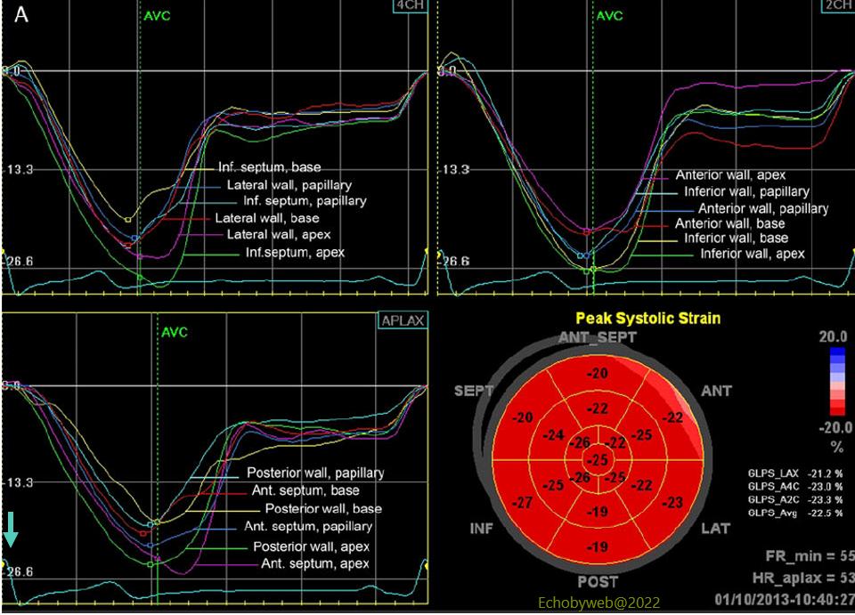
Figure 1. The AFI algorithm calculates the % strain negative value (the small colored squares mark the maximum segmental contraction) between the ECG R wave (light blue arrow) and end-ejection (green dotted line). In each view, six wall segment lines are analysed (total= 18 segments), whereas the bull’s eye graph show a LV 17-segment model averaging apical segments and extrapolating the true apex. In this normal example all segmental longitudinal strain curves peak at end-ejection.
AVC= aortic valve closure; FR; frame rate; HR; heart rate; GLPS_Avg: Average calculated Global Longitudinal Peak Strain (systolic).
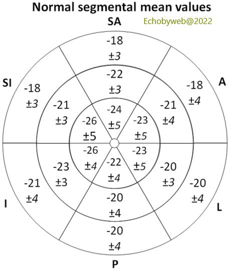
Normal regional values:
Base segments= – 18.9 ± 2.4 %
Mid (papillary) segments= -21.3 ± 2.2 %
Apical segments= – 24.3 ± 2.2 %
Population sample from:
Barbier P. Eur Heart J Cardiovasc Imaging 2015